Quickstart

This page provides an example of how to perform a single VPLanet simulation. It introduces you to the input and output files, executing the simulation, and visualizing the result with vplot. This example, however, only represents a small fraction of the VPLanet use cases, so it is intended to be representative of how to use the code. In other words, the files shown below represent the typical structure, formatting and syntax for all VPLanet simulations. Understanding this example will enable you to build off the other examples included in this repository.

Physics of the Example

Let’s go over how to use VPLanet by simulating the evolution of water on Venus. Isotopic evidence suggests Venus may have had a similar amount of water to Earth in the past (Donahue et al., 1982), but because of vigorous hydrodynamic escape it may have lost all of it in the first few hundred Myr (Hunten, 1973). Here we’re going to use the stellar and atmesc modules of VPLanet to jointly model the evolution of the Sun and Venus in order to estimate how long it took for Venus to lose all its surface water.

Note

This guide shows how to interpret the VenusWaterLoss example, but here we will only include one planet, whereas the example uses three. Modifying that example to match the input files shown below will generate the figure at the end of this guide.

The basic workflow for a VPLanet simulation is to 1) create input files with the relevant system, star, and/or planet parameters, 2) execute VPLanet directly from the command line, and 3) interpret the ASCII text output generated in a log file and/or time-series data file.

The Input Files

VPLanet takes 1 file as input, which contains “options” that direct the execution of the code. Each option is defined by a single, case-sensitive name, and is followed by one or more arguments. The option file included in the command line is called the “primary input file” and provides VPLanet with the most general information about the simulation, e.g. the integration method, the stop time, what bodies are in the system, etc. It also must include a list of files that contains information about the bodies in the system, called the “body files.”

This primary input file is usually called vpl.in, but you can call it whatever you’d like. We’ll start by presenting an example, and then dissect it after. The primary input file generally takes a form like this:

vpl.in

# General Options
sSystemName   solarsystem        # System Name
iVerbose      5                  # Verbosity level
bOverwrite    1                  # Allow file overwrites?
saBodyFiles   sun.in $           # List of all bodies files for the system
              venus.in           # The $ tells VPLanet to continue to the next line

# Input/Output Units
sUnitMass      solar             # Options: gram, kg, Earth, Neptune, Jupiter, solar
sUnitLength    AU                # Options: cm, m, km, Earth, Jupiter, solar, AU
sUnitTime      YEARS             # Options: sec, day, year, Myr, Gyr
sUnitAngle     d                 # Options: deg, rad

# Input/Output
bDoLog         1                 # Write a log file?
iDigits        6                 # Maximum number of digits to right of decimal

# Evolution Parameters
bDoForward    1                  # Perform a forward evolution?
bVarDt        1                  # Use variable timestepping?
dEta          0.01               # Coefficient for variable timestepping
dStopTime     4.6e9              # Stop time for evolution
dOutputTime   1e6                # Output interval for forward files

Note

You can obtain descriptions of the options from the command line with the -h (short help) or -H (long help) flags. You can also search the options here.

As described above, the options are specified with a unique string (e.g., dEta or dStopTime) followed by white space and then the value(s) for the option. Note that the leading lower case letter(s) of each option’s name describes the type (or “cast”) of the expected argument: b = Boolean, i = integer, d = double precision, s = string. If an “a” follows one of these letters, then the argument may contain multiple values, i.e. may be an “array,” e.g. saBodyFiles on line 5. Only one option is allowed per line.

The order of the options is irrelevant, and white space is ignored. Comments can be specified anywhere with the hashtag (#) symbol. Note that array options can span multiple lines with the $ symbol, as shown in the arguments to saBodyFiles. The $ tells VPLanet to find the next member of the array on the next line. The # and $` symbols are the only special characters in VPLanet input files.

The name of each option is intended to be helpful, i.e. self-explanatory, but here’s a line-by-line breakdown to be clear (ignoring comments and white space): We’re calling the system "solarsystem", which automatically sets the names of output files to use the argument as the prefix, as well as enable vplot to easily use the name. We specified maximum verbosity (5), so VPLanet will talk a LOT. We’re allowing output file overwrites. Next we get to the all important list of body files, and we’re telling the code to expect two that are called sun.in and venus.in, which we’ll describe below. (Note that in the VenusWaterLoss example, three planets are simulated, each representing a different amount of initial water content.) Next, we set the default units for I/O: solar masses, astronomical units, years, and degrees. Because we set them in the primary input file, the choices are propagated to the body files, but a user can specify units for each body. In the case of some double precision options, the user can also force specific units with a negative sign, as described below.

Next, bDoLog tells the code to generate a log file; iDigits sets the output precision to 6 decimal places. The last block of options tells VPLanet how to simulate the system. We want to evolve the system forward in time. We will employ variable (adaptive) timestepping with, as set in the next line, the accuracy coefficent dEta set to 0.01, i.e. the code will set the time step to be 100 times shorter than the time required for the value of the fastest changing variable to change by a factor of 2. The final two lines specify the length of the integation (in units of sUnitTime), and the frequency of outputs.

Note

The smaller the value of dEta, the higher the precision of the integration, but the slower it will run. We have found that many cases converge for a value of 0.01, but some require 0.0001. Always test for convergence before assuming VPLanet output is accurate.

With the primary input file completed, let’s now turn to the two body files, sun.in and venus.in.

sun.in

# Star's Parameters
sName           sun              # Body's name
saModules       stellar          # Modules to apply, exact spelling required

# Physical Parameters
dMass           1.00             # Mass of the star in solar masses
dAge            5e7              # Age in years at integration start

# STELLAR Parameters
sStellarModel   baraffe          # Stellar evolution model: `baraffe` or `none`
dSatXUVFrac     1.e-3            # XUV luminosity fractional saturation level
dSatXUVTime     1e8              # XUV saturation timescale in years

# These are the parameters that vplanet will output as arrays in the
# `.forward` or `.backward` evolution files. Run `vplanet -h` for a list
# of all options. Note that the "-"" sign creates output with custom units.
saOutputOrder   Time -LXUVStellar

As before, the parameter names are intended to be self-explanatory. Note that we’re only setting a few, and those that are not specified assume their default values. Here we have a few differences with VenusWaterLoss: That example assigns a hexadecimal color that can be used for plotting with vplot, and uses the negative option for dSatXUVTime, which means the units are Gyr. For this guide, we’re running a shorter integration.

We gave the star a name and told VPLanet we want to use the stellar module to compute its evolution. We assigned its mass and age at simulation time = 0, and set a few stellar-specific properties. We’ll use the Baraffe et al. (2015) evolutionary tracks and the Ribas et al. (2005) XUV evolution power law with a saturation fraction of 0.001 and saturation time of 100 Myr. Note that “time” is different than “age” in that the former is the internal counter for the simulation, whereas the latter is the physical age of the star since some birth time. For a compete description of the physics in VPLanet, please consult the manual.

The option saModules is of particular importance in the body files as it sets the physical models (“modules”) to be applied to the body. In this case, the only module is “stellar”, or the quiescent evolution of a star from formation to the end of the hydrogen burning. In more complicated simulations, multiple modules can be added to the argument list and the code will automatically add the new equations, including coupling of any parameters that are affected by multiple modules.

Another important VPLanet option is saOutputOrder, which is a list of all parameters to be output during the integration at a cadence defined by dOutputTime (see vpl.in, line 23). In this case we requested two “outputs”: time and XUV luminosity. (The example includes a few more parameters.) Output names need only be unique, unlike the option names, but it’s often easier to understand the output if the full name is provided. As shown below, the log file contains the list of outputs and their units for each body.

Note

Some output parameters (usually those that are positive-definite) can be prepended with a minus sign to force the output into a customized unit. This information can also be found in the help file. In general these “custom units” are tailored to the Sun-Earth system.

Next up is the input file for the planet, Venus. This example is based off venus1.in in VenusWaterLoss.

venus.in

# Planet's Parameters
sName            venus           # Body's name
saModules        atmesc          # Modules to apply, exact spelling required
saOutputOrder    Time $
                 -SurfWaterMass $
                 -OxygenMantleMass

# Physical Parameters
dMass         -0.815             # Here, the - symbol means Earth masses
dRadius       -0.9499            # Here, the - symbol means Earth radii
dSemi         0.723              # Semi-major axis
dEcc          0.006772           # Eccentricity

# ATMESC Parameters
dSurfWaterMass       -1.0        # Initial surface water in Earth oceans
sWaterLossModel      lbexact     # Water loss model; Luger and Barnes (2015)
bInstantO2Sink       1           # O2 is absorbed instantly at the surface
sAtmXAbsEffH2OModel  bolmont16   # XUV absorption efficiency model

This file looks pretty similar to the previous one, but it’s worth noting a few things. First, we appear to have given the planet a negative mass and radius! As mentioned above, the negative sign is actually telling VPLanet to apply different units. Many parameters have an associated customized unit that overrides the default units specified in vpl.in. In this case, dMass and dRadius have customized units of Earth masses and Earth radii, respectively, so we’re OK.

Similarly, note that two outputs have a negative sign in front of them. These symbols tell VPlanet to output to this parameter to the data files in custom units.

Finally, we set some atmesc-specific parameters. We told the code to initialize the planet with one Earth ocean’s worth of water (the minus sign, again, indicates custom units) and to compute the water loss using the model from Luger and Barnes (2015) and oxygen be absorbed at the surface instantly. The sWaterLossModel employs the XUV absorption efficiency model from Bolmont et al. (2016).

Running the Code

Now that you understand how the input files work, we are ready to run the code!

vplanet vpl.in

Upon running this command in a terminal, you may see all sorts of messages printed to the screen:

INFO: sUnitMass set in vpl.in, all bodies will use this unit.
INFO: sUnitTime set in vpl.in, all bodies will use this unit.
INFO: sUnitAngle set in vpl.in, all bodies will use this unit.
INFO: sUnitLength set in vpl.in, all bodies will use this unit.
INFO: sUnitTemp not set in file sun.in, defaulting to Kelvin.
INFO: sUnitTemp not set in file venus1.in, defaulting to kelvin.
INFO: sUnitTemp not set in file venus2.in, defaulting to kelvin.
INFO: sUnitTemp not set in file venus3.in, defaulting to kelvin.
INFO: dRotPeriod < 0 in file sun.in, units assumed to be Days.
INFO: dMass < 0 in file venus.in, units assumed to be Earth masses.
INFO: dSemi < 0 in file venus.in, units assumed to be AU.
INFO: dRadius < 0 in file venus.in, units assumed to be Earth radii.
INFO: dRotPeriod < 0 in file venus.in, units assumed to be Days.
INFO: dSurfWaterMass < 0 in file venus.in, units assumed to be Terrestrial Oceans (TO).
INFO: dMinSurfWaterMass < 0 in file venus.in, units assumed to be Terrestrial Oceans (TO).
INFO: dJeansTime not set for body venus, defaulting to 3.16e+16 seconds.
Input files read.
INFO: Age set in one file, all bodies will have this age.
INFO: sOutFile not set, defaulting to solarsystem.sun.forward.
INFO: sOutFile not set, defaulting to solarsystem.venus.forward.
INFO: sIntegrationMethod not set, defaulting to Runge-Kutta4.
INFO: dEnvelopeMass < dMinEnvelopeMass. No envelope evolution will be included.
INFO: dEnvelopeMass < dMinEnvelopeMass. No envelope evolution will be included.
INFO: dEnvelopeMass < dMinEnvelopeMass. No envelope evolution will be included.
INFO: Radius of Gyration set for body 0, but this value will be computed from the grid.
All of sun's modules verified.
All of venus's modules verified.
Input files verified.
Log file written.

You can safely ignore most of this output: VPLanet is just being very verbose (as requested!) about what it’s doing. It is, however, a good idea to examine those messages to ensure you haven’t made any mistakes! If VPLanet thinks you’re doing something dubious, it will output a WARNING and you should take care that you are comfortable with your options. VPLanet will also ERROR in cases of incompatible options, values out of bounds, etc., and provide the file and line number(s) that contain the issue(s). Note that if you did run the examples/VenusWaterLoss case you will see more Venuses in the output.

Anfter informing you of many of the decisions VPLanet made, things will go silent for a couple seconds, and then you’ll see:

Evolution completed.
Log file updated.
Simulation completed.

The code is done running, and you should see several output files in the current directory.

The Output Files

The log file records the details of the simulation and captures a snapshot of the system at the initial step and the final step of the evolution. Here’s a very condensed version of what you should see:

solarsystem.log

Executable: vplanet
Version: <GITVERSION>
System Name: solarsystem
Primary Input File: vpl.in
Body File #1: sun.in
...

---- INITIAL SYSTEM PROPERTIES ----
(Age) System Age [sec]: 1.577880e+15
(Time) Simulation Time [sec]: 0.000000
...
----- BODY: sun ----
Active Modules: STELLAR
(Mass) Mass [kg]: 1.988416e+30
...
----- STELLAR PARAMETERS (sun)------
(LXUVStellar) Base X-ray/XUV Luminosity [LSUN]: 0.000677
Output Order: Time[year] LXUVStellar[LSUN]

----- BODY: venus ----
Active Modules: ATMESC
(Mass) Mass [kg]: 4.867332e+24
...
----- ATMESC PARAMETERS (venus)------
(SurfWaterMass) Surface Water Mass [TO]: 1.000000
...
Output Order: Time[year] SurfWaterMass[TO] OxygenMantleMass[bars]

---- FINAL SYSTEM PROPERTIES ----
(Age) System Age [sec]: 1.467428e+17
(Time) Simulation Time [sec]: 1.451650e+17
...
----- BODY: sun ----
Active Modules: STELLAR
(Mass) Mass [kg]: 1.988416e+30
...
----- STELLAR PARAMETERS (sun)------
(LXUVFrac) X-ray/XUV Luminosity Fraction []: 8.892684e-06
...
----- BODY: venus ----
Active Modules: ATMESC
(Mass) Mass [kg]: 4.867332e+24
----- ATMESC PARAMETERS (venus)------
(SurfWaterMass) Surface Water Mass [TO]: 0.000000
(OxygenMantleMass) Mass of Oxygen in Mantle [bars]: 199.365415
...

The log file lists parameter values in system units: SI. This choice allows users to be sure that all the calculations will proceed correctly. Note, however, that any output given a negative sign prefix will appear in the custom units. Also note that the log file contains the complete initial and final conditions for all outputs for the selected modules. The first word in many of the log file lines is in parentheses, which indicates the parameter can be supplied to saOutputOrder to record the evolution over time.

Next, we will consider the output files, one per body, which are often called “forward files” or “backwards files”. The columns in these files correspond to names in the saOutputOrder option in the corresponding input files. Recall that for the Sun, we requested that VPLanet output the simulation time and the XUV luminosity (in solar units since we used the minus sign):

solarsystem.sun.forward

0.000000     0.000677
1.000000e+06 0.000677
2.000000e+06 0.000678
3.000000e+06 0.000678
4.000000e+06 0.000678
...

Currently forward files do not include headers, but you can verify the outputs columns and their units in the log file. For the planet, we asked for the time, the amount of surface water (with a minus sign, indicating in units of Earth oceans), and the amount of oxygen absorbed by the mantle (with a minus sign, indicating units of bars):

solarsystem.venus.forward

0.000000     1.000000 0.000000
1.000000e+06 0.978763 4.238860
2.000000e+06 0.957524 8.477719
3.000000e+06 0.936283 12.716579
4.000000e+06 0.915044 16.955439
...

Plotting

With the output generated, it is often convenient to plot the output. While any plotting package can be used, the VPLanet team has created a customized tool that enables both fast plotting of output, as well as tools to generate publication worthy figures. The vplot tool (docs here) can be used to easily visualize the results of any VPLanet simulation. After VPLanet finishes, simply run

vplot

for the a plot like the following to appear:

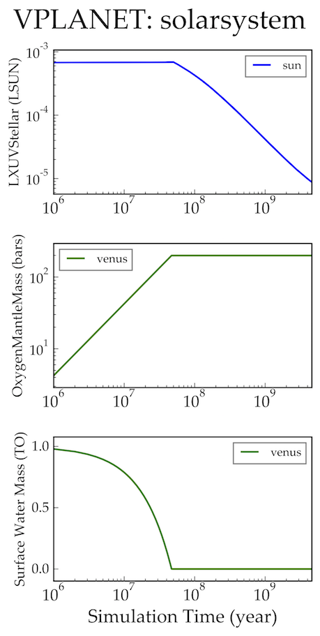
vplot plots the time series of all the variables from all the bodies in a single figure. Here we see the evolution of the stellar XUV emission, which declines dramatically after the saturation timescale ends (top); the increase in the amount of oxygen in the planet’s mantle, which is absorbed from the oxygen released from the photolysis of water (center); and the desiccation of the planet’s surface, caused by the hydrodynamic escape of hydrogen to space. In this simulation, Venus loses all of its surface water in about 50 Myr.

Next Steps

The above example describes one use case, but VPLanet can simulate many more phenomena, all with the same executable and input file format. Navigate to the examples directory to see the physics that are currently available. Each example provides instructions on how to generate output and a figure.

Also available are Python scripts for generating parameter sweeps and storing the data from those sweeps. See the parameter sweep guide for more details.